Paper summary
ReversoEfficient Time Series Foundation Models for zero-shot forecasting
Live demo · Paper · Code · Models · Correspondence
Summary
Time series foundation models are often scaled to hundreds of millions—or even billions—of parameters. Reverso asks a simpler question: how small can a general-purpose forecasting model be while remaining competitive?
Reverso combines multi-scale inputs, long convolutions, DeltaNet layers, and an attention-based decoder. The largest model has only 2.6 million parameters, yet reaches a 0.706 MASE on the full Gift-Eval benchmark and performs strongly across forecasting, classification, anomaly detection, imputation, and probabilistic forecasting.
1. Motivation
Foundation models make it possible to forecast an unfamiliar time series without task-specific training. But most progress has followed the scaling playbook from language and vision: train a larger model on more data. That makes strong forecasters harder to deploy on-device, at the edge, or anywhere memory and latency matter.
Reverso explores the opposite direction. It keeps the architecture compact, uses efficient sequence-mixing primitives, and adds practical training and inference strategies that improve accuracy without requiring a large transformer.
| Model | Parameters | Layers | Width |
|---|---|---|---|
| Reverso-Nano | 200K | 2 | 32 |
| Reverso-Small | 550K | 4 | 64 |
| Reverso | 2.6M | 8 | 128 |
2. Architecture
A Reverso block alternates two efficient ways of mixing information across time: long convolutions capture broad patterns in parallel, while DeltaNet layers maintain a recurrent state for sequential dependencies. Each sequence mixer is followed by a small MLP for channel mixing.
The input is represented at four temporal scales. Each scale looks farther back in time through progressively stronger downsampling, so the model receives up to 16,384 historical points while processing a sequence of length 2,048. An attention-based decoder then predicts 48 future points at a time.
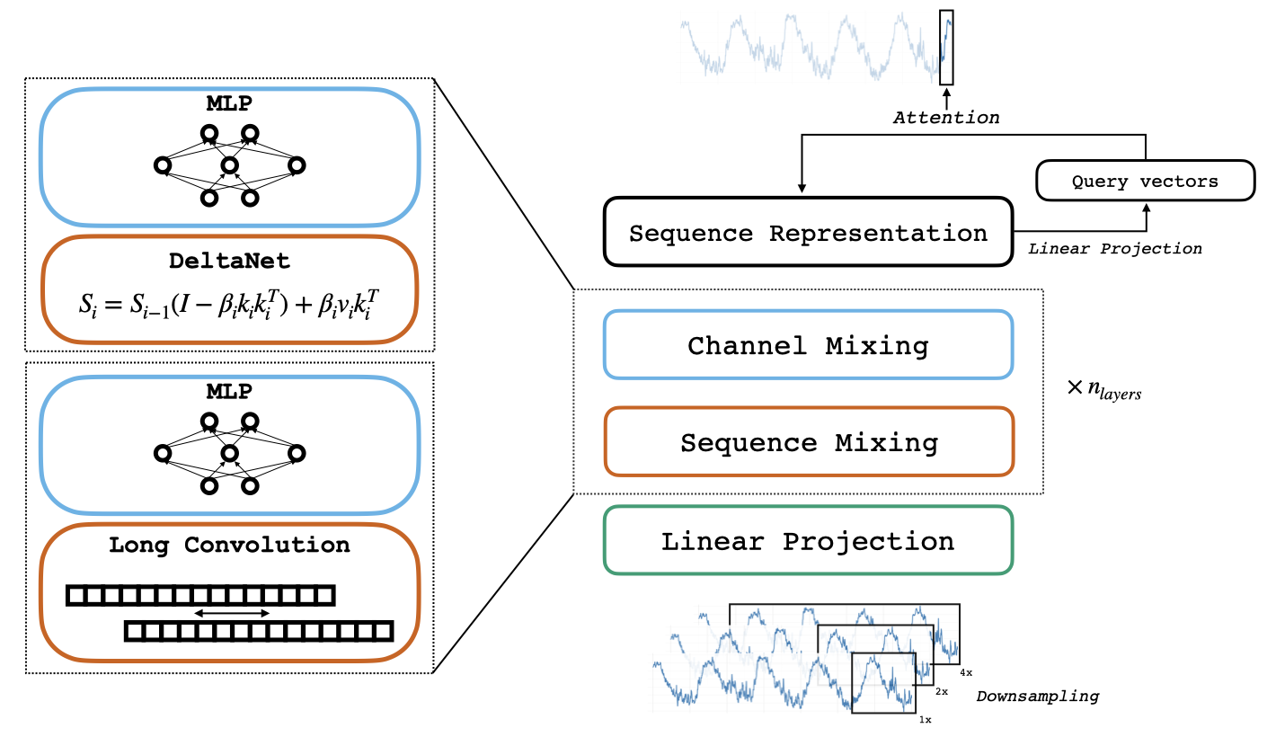
- Multi-scale context. Four downsampled views expose both recent detail and long-range structure.
- Hybrid sequence mixing. Long convolutions and DeltaNet layers alternate throughout the model.
- Attention decoder. Learned output queries attend to the encoded history and predict the next 48 points.
3. Training recipe
The models are pretrained on heterogeneous real and synthetic time series. The data pipeline combines standard augmentations—including mixup, downsampling, censoring, and amplitude modulation—with Gaussian-process, spike-process, and TSI synthetic sequences.
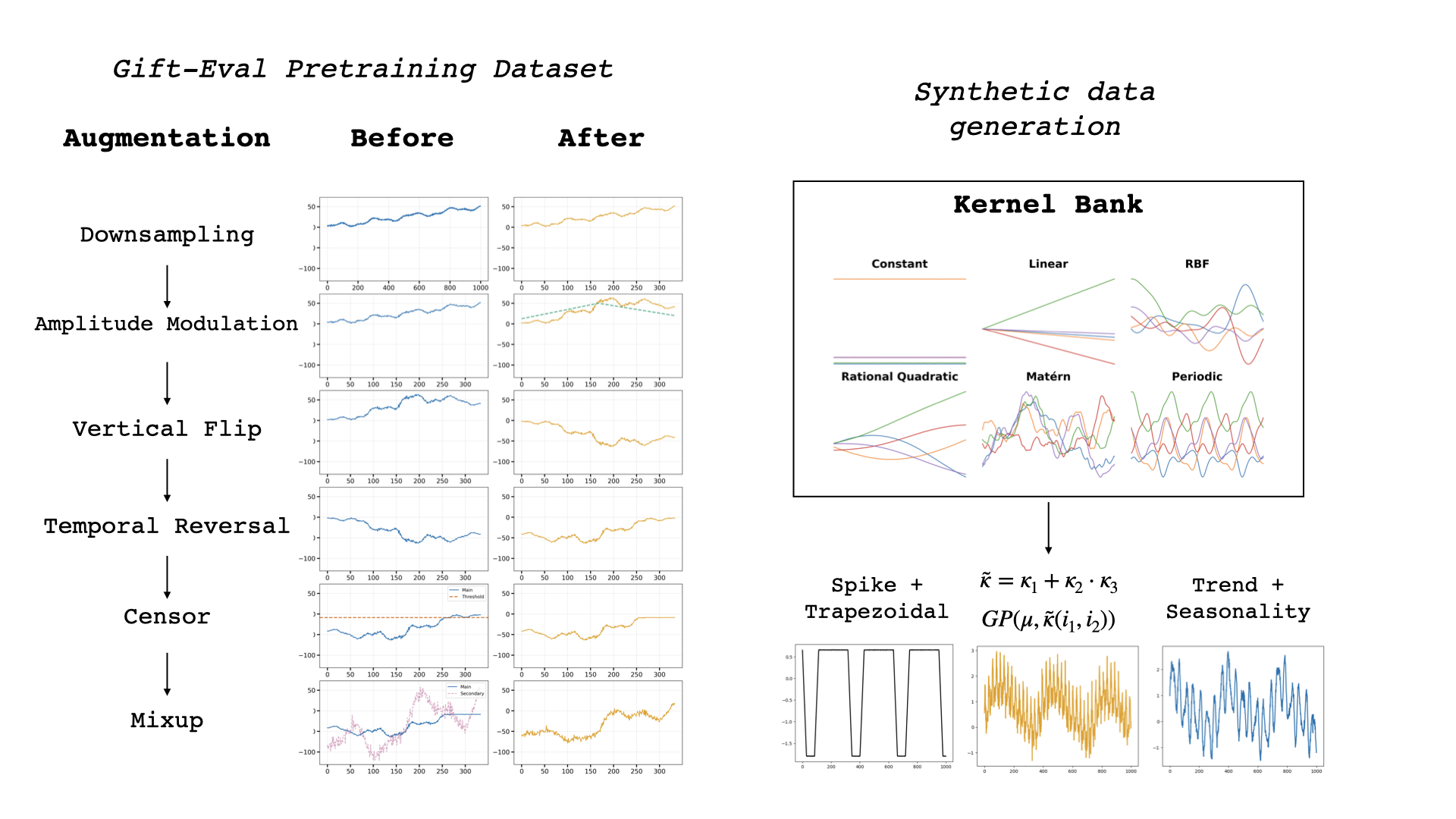
Full training takes roughly 10, 20, and 40 H100-hours for Reverso-Nano, Reverso-Small, and Reverso respectively. An FFT-based downsampling rule also compresses very long seasonal patterns when their period exceeds the model context.
4. Forecasting results
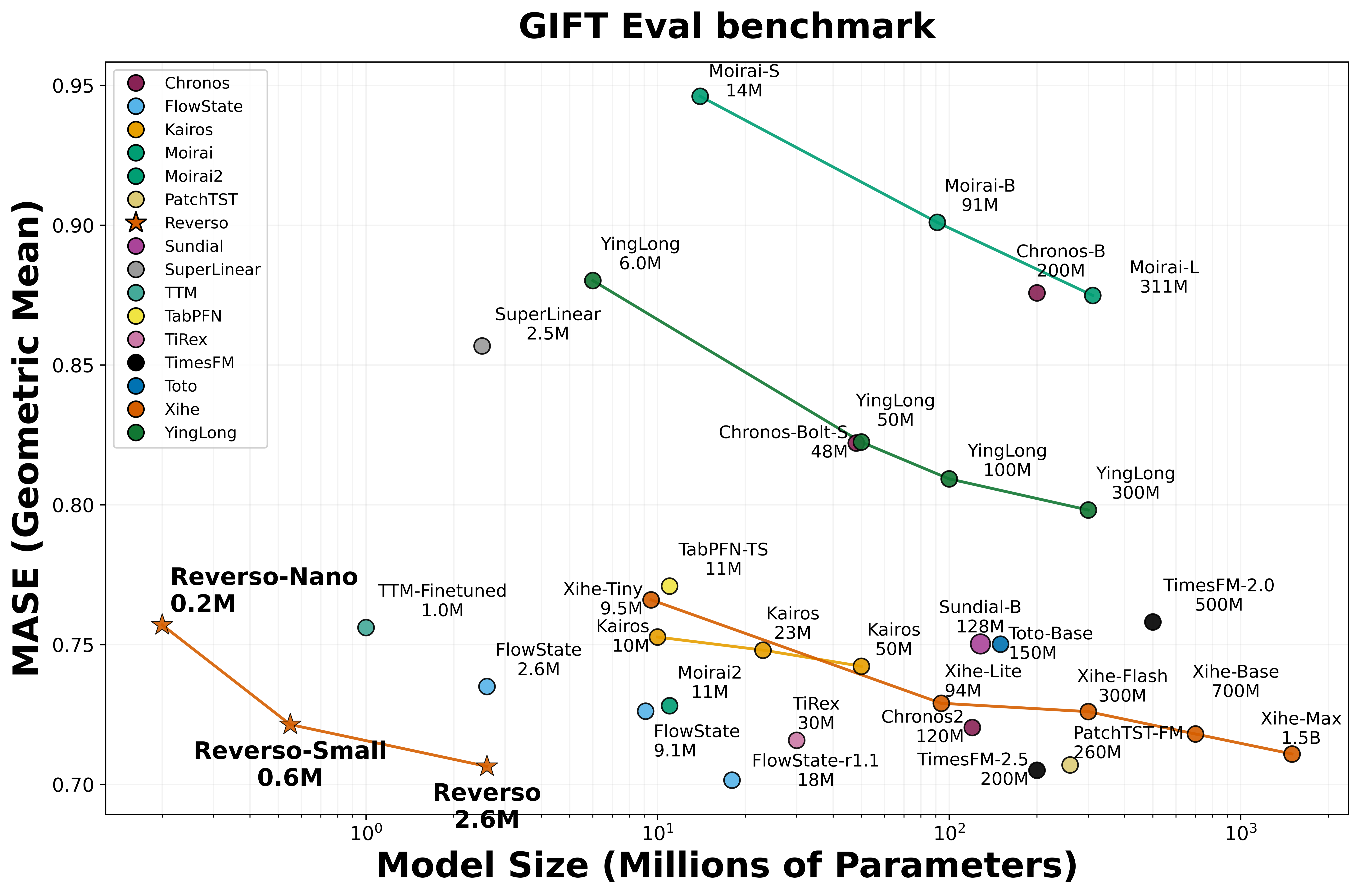
Gift-Eval spans 97 forecasting tasks from 23 datasets across seven domains. Reverso reaches 0.706 overall MASE with 2.6M parameters, outperforming similarly sized models and closely tracking much larger systems.
| Model | Parameters | MASE ↓ |
|---|---|---|
| FlowState-r1.1 | 18M | 0.701 |
| TimesFM-2.5 | 200M | 0.705 |
| Reverso | 2.6M | 0.706 |
| Xihe-Max | 1.5B | 0.711 |
On the 21 long-sequence Gift-Eval datasets with all three horizon lengths, Reverso has the best average MASE in the reported comparison: 0.691. It is especially strong at medium and long horizons despite forecasting autoregressively in 48-point chunks.
| Model | Short | Medium | Long | Average |
|---|---|---|---|---|
| PatchTST-FM | 0.616 | 0.722 | 0.745 | 0.694 |
| FlowState-r1.1 | 0.633 | 0.720 | 0.736 | 0.696 |
| Reverso | 0.634 | 0.699 | 0.741 | 0.691 |
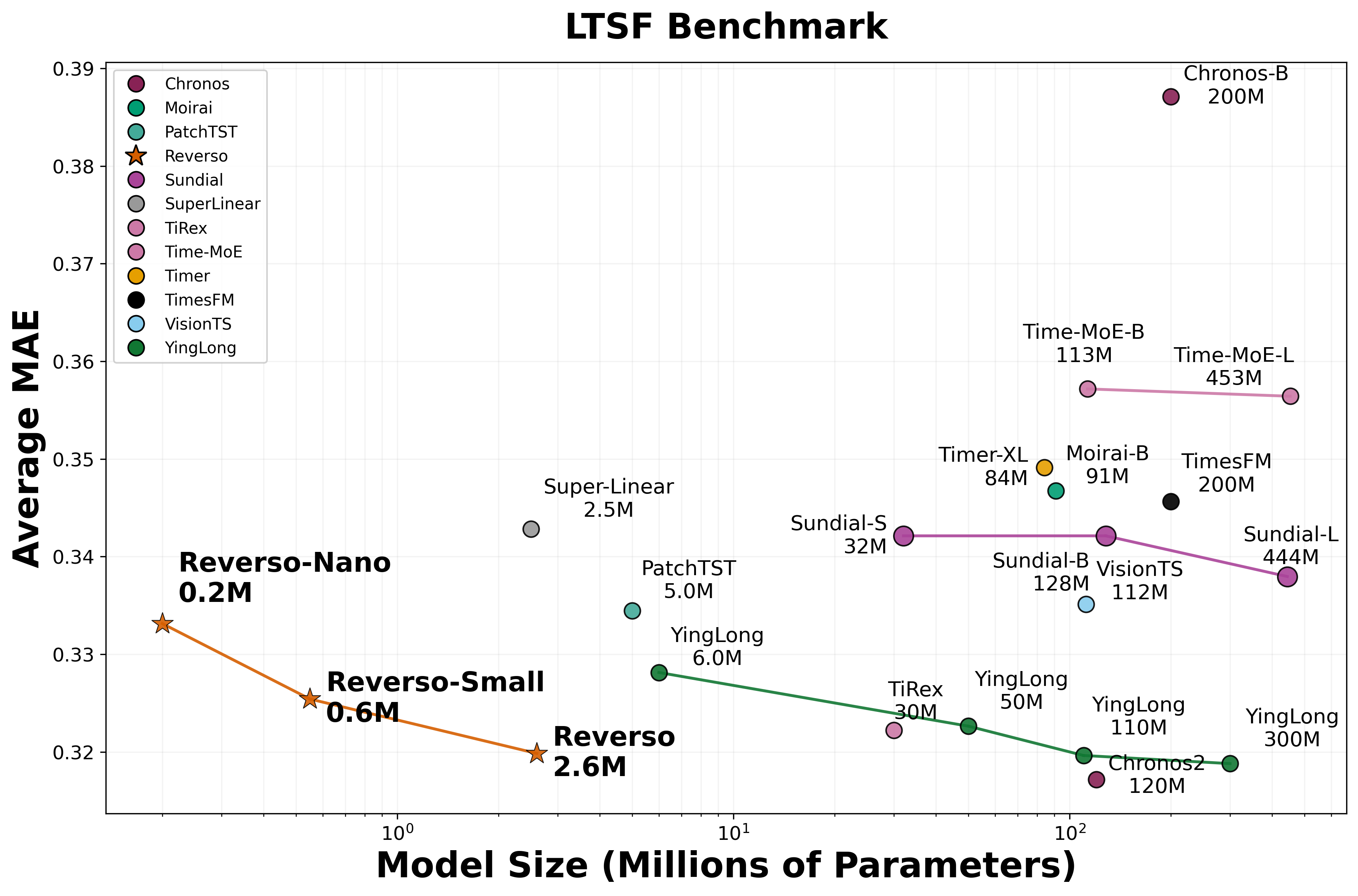
Reverso also transfers well to the LTSF benchmark, averaging 0.322 MAE across six datasets and four prediction horizons—competitive with models tens or hundreds of times larger.
5. Beyond forecasting
Although trained primarily as a univariate forecaster, Reverso learns representations that transfer to other time-series tasks.
| Model | Parameters | UCR | Multivariate UEA |
|---|---|---|---|
| Reverso | 2.6M | 81% | 74% |
| TiRex | 30M | 81% | 74% |
| Chronos-Bolt | 205M | 79% | 74% |
On zero-shot UCR anomaly detection, Reverso detects 88, 126, and 188 labeled anomalies when the top 1%, 3%, and 10% of forecast-error segments are flagged. It also achieves the best reported imputation MSE on all seven tested datasets, and its pretrained backbone supports competitive probabilistic forecasts after training a quantile-regression decoder.
These downstream evaluations use lightweight task-specific protocols: a frozen encoder plus random forest for classification, forecast error for anomaly detection, and fine-tuned heads for imputation and probabilistic forecasting.
6. Efficiency
Parameter efficiency
Reverso reaches competitive zero-shot forecasting accuracy with only 2.6 million parameters. It is roughly 77 times smaller than TimesFM-2.5 and more than 570 times smaller than Xihe-Max, while remaining on the Gift-Eval and LTSF performance-efficiency frontiers.
Latency efficiency
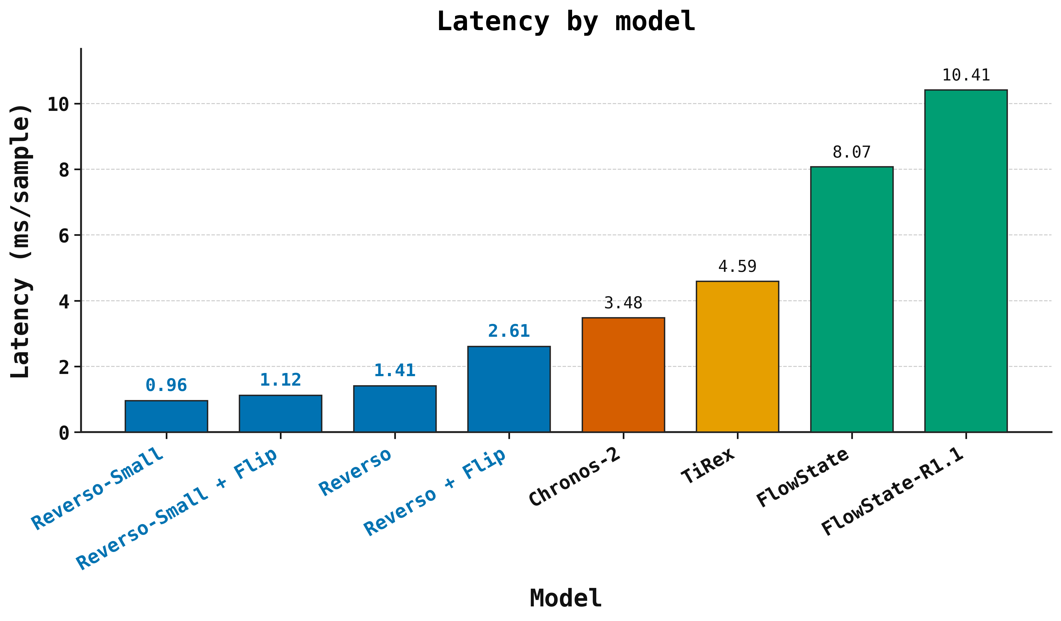
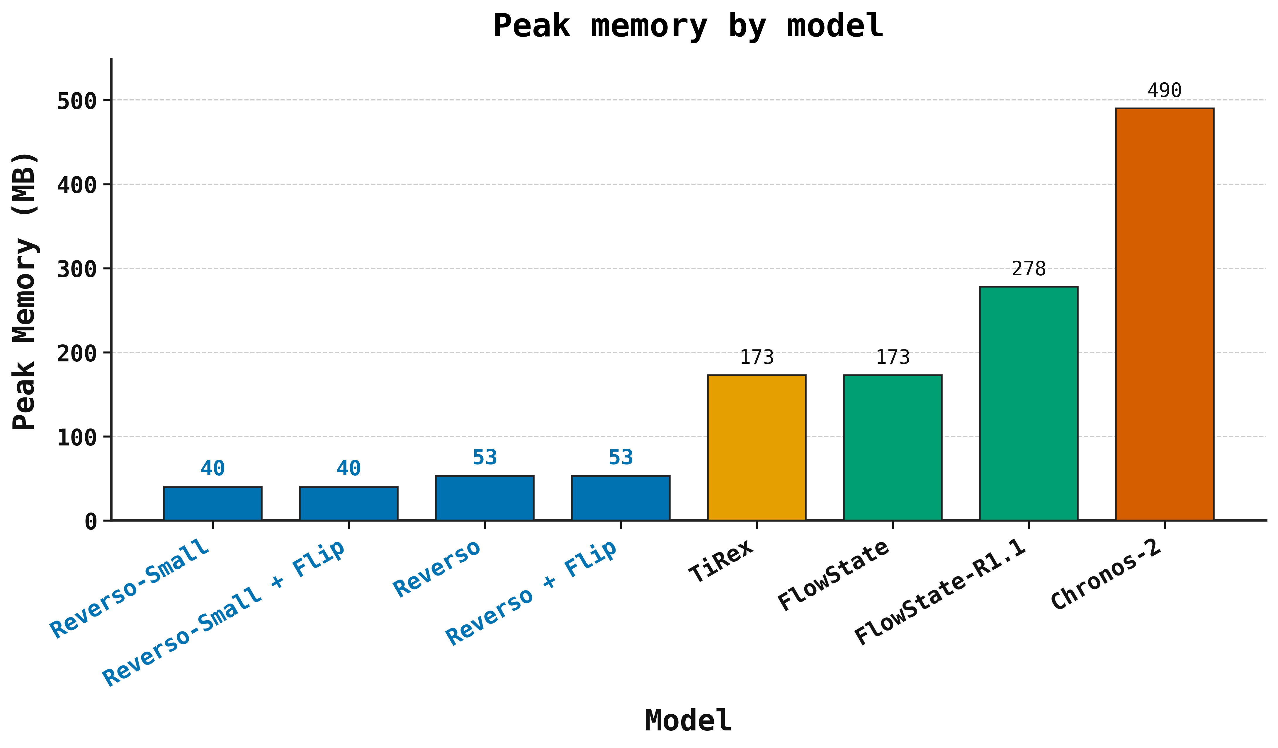
The compact parameter count translates into practical inference efficiency. On a single H100, Reverso variants achieve lower latency and use less peak memory than much larger time series foundation models while staying on the performance frontier.
7. Limitations
Several limitations remain:
- Reverso is trained primarily as a univariate forecaster and does not explicitly model cross-channel dependence.
- Short-sequence performance still trails the strongest large models on some tasks.
- The base model produces point forecasts; probabilistic forecasts require an adapted decoder objective.
- Some efficiency measurements use an H100 and may differ on edge-class hardware.
Citation
@misc{fu2026reverso,
  title   = {Reverso: Efficient Time Series Foundation Models
             for Zero-shot Forecasting},
  author  = {Fu, Xinghong and Li, Yanhong and Papaioannou,
             Georgios and Kim, Yoon},
  year    = {2026},
  eprint  = {2602.17634},
  archivePrefix = {arXiv}
}